How a handful of (noisy) points becomes a predictive distribution, and how that distribution becomes a strategy for finding x^* at the lowest possible computational (experimentation) budget.

Every engineering design loop hides the same villain: a simulation that is accurate but slow. A CFD run on a wing can take eight hours on 64 cores; a crash simulation, longer still. Gradient-based optimizers want hundreds of such calls, uncertainty quantification wants thousands, and design-space exploration wants more stillSee the "online vs. offline cost" and "break-even" discussion later in this article — with a representative external-aerodynamics case, a single high-fidelity run costs on the order of $20, and a converged optimization needs 60–130 of them.. The standard answer is a surrogate model: a cheap, differentiable stand-in \hat{y}(x) trained on a small design of experiments, used in place of the expensive code inside an optimization loop.

This article builds that idea from scratch and ends where a lot of real design optimization currently lives: Bayesian Optimization — using a Gaussian Process not just to predict, but to decide where to sample next under a tight budget. Every figure below is generated by the same code as the source notebooks (linked throughout), and the two boxed panels are fully interactive — drag points, change kernels, click to sample a "black box," and watch the algorithm choose its next move.

Part 1 — What is a Gaussian Process?

The idea has two independent histories that turned out to be the same idea. In 1951, mining engineer Daniel Krige proposed a statistical method for estimating gold concentration between boreholes on the Witwatersrand ; Georges Matheron formalized it at Mines of Paris in the 1960s as kriging . Few years later, in the machine-learning world, Radford Neal showed in 1994 that a neural network with an infinite number of hidden units converges to a Gaussian Process — the same mathematical object, arrived at from another direction. Today "kriging" and "Gaussian Process regression" are the same computation with different vocabularies: geostatisticians say \theta, machine learners say hyperparameters; one side calls it the variogram, the other the kernel.

Here is the problem a GP solves, verbatim from the running example in this article (adapted from Ebden's 2008 tutorial , and the exercise in GP_tutorial.ipynb): given six noisy observations \{(x_i, y_i)\}_{i=1}^{6}, what is the best estimate of y at a new point x_* — including at a point outside the training range, where we are extrapolating rather than interpolating?
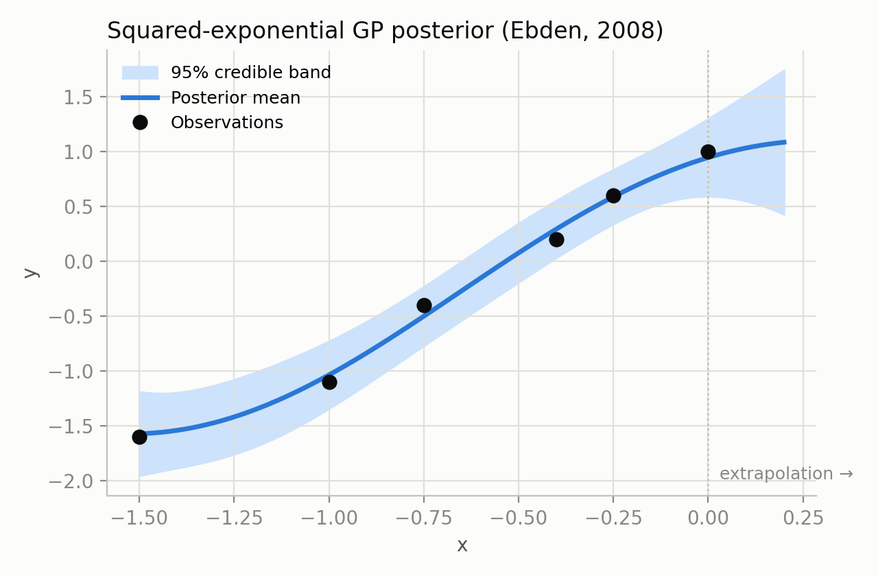
GP posterior mean and 95% credible band fit to six points with a squared-exponential kernel
The posterior mean (blue) and 95% credible band (shaded) of a GP fit to six points with a squared-exponential kernel, \ell=1, \sigma_f^2=\sqrt{3}, \sigma_n=0.2 — exactly the numbers chosen in GP_tutorial.ipynb. Notice the band widens past x=0: the model knows what it doesn't know.

A Gaussian Process is a distribution over functions such that any finite collection of function values is jointly Gaussian. It is fully specified by a mean function (we take it to be zero, after centering the data) and a covariance — or kernel — function k(x, x') that encodes how strongly two outputs should co-vary given how far apart their inputs are. The workhorse choice, the squared-exponential (also called RBF or Gaussian) kernel, is

k(x, x') = \sigma_f^2 \exp\!\left(-\frac{(x - x')^2}{\ell^2}\right) + \sigma_n^2\,\delta_{ij}

with three hyperparameters: the length-scale \ell (how quickly correlation decays with distance — the "wiggliness"), the signal variance \sigma_f^2 (the vertical scale of the function), and the noise variance \sigma_n^2 (how much we distrust each observation). Stack the training inputs into \mathbf{X} and evaluate the kernel pairwise to build the Gram matrix K; the training outputs and the unknown value at x_* are then jointly Gaussian:

\begin{bmatrix} \mathbf{y} \\ y_* \end{bmatrix} \sim \mathcal{N}\!\left(\mathbf{0}, \begin{bmatrix} K & K_*^\top \\ K_* & K_{**} \end{bmatrix}\right)

Conditioning a joint Gaussian on part of itself is elementary — it is the same "Schur complement" trick used for regression coefficients in linear-Gaussian models — and it gives closed-form expressions for the posterior mean and variance at any x_*:

\bar{y}_* = K_* K^{-1} \mathbf{y}, \qquad \mathrm{var}(y_*) = K_{**} - K_* K^{-1} K_*^\top

That is the entire algorithm: build two small matrices, invert one of them (in practice, via a Cholesky factorization for numerical stability — K becomes ill-conditioned when points sit close together, which is why production libraries use the partitioned/Cholesky route rather than a naive K^{-1}), and multiply. No neural network, no iterative training loop — everything here is analytical and exact, which is exactly why GPs are the workhorse surrogate in low-data, low-to-medium-dimensional engineering design, where a neural network would be starved of data and would not report calibrated uncertainty .

Play with it. The panel below implements exactly the equations above — four kernels, three hyperparameters, live. Drag a point, switch the kernel, or click empty space to add an observation and watch the credible band react. The "Fit ℓ, σ_f by max. likelihood" button does a grid search over \log p(\mathbf{y} \mid \mathbf{X}, \theta) — the same objective used to tune hyperparameters in every production GP library (SMT, EGObox, scikit-learn). The two small panels below the plot are the notebook's own plt.imshow(covXXs) and plt.imshow(covXX_noisy) cells, live — watch the Gram matrix reorganize as you drag points around (nearby points in x stay bright/correlated regardless of where you drag them, since the kernel only sees distance). Tick "show posterior samples" to draw random function draws from the posterior, exactly like the notebook's L.T @ np.random.randn(N, 5) cell.

Part 2 — Choosing a kernel, and why the "right" one is not obvious

The kernel is a modeling choice, not a fact about the data, and different kernels extrapolate very differently from the same six points. GP_tutorial_2.ipynb compares four options available in SMT's KRG surrogate — squared-exponential, exponential (Ornstein–Uhlenbeck i.e. OU), Matérn 3/2 and Matérn 5/2 — fit to the identical training set, then evaluated at an extrapolation point just outside the training range:
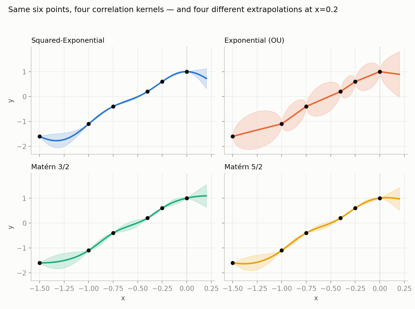
Four kernels fit to the same six points, with very different extrapolation behavior and uncertainty past x=0
Squared-Exponential — infinitely smooth, can over-commit Exponential (OU) — rough, widens fastest Matérn 3/2 — once-differentiable, a common default Matérn 5/2 — twice-differentiable, a common default
Same six points, four correlation functions. The mean prediction and — more importantly — the width of the 95% band at the unseen point x=0.2 differ meaningfully across kernels. There is no universally "correct" kernel; see Duvenaud's kernel cookbook for a field guide to composing and choosing them.
Play with it. The static figure fixes one dataset; this panel lets you change it. Drag the six points and all four kernels refit themselves — independently, by maximizing their own log marginal likelihood — so you can watch, live, how each one's extrapolation and uncertainty diverge as the data gets sparser, noisier, or more clustered. Drag the orange x_* marker to slide the "unknown" query point anywhere, including well outside the training range, and read off each kernel's 95% interval in the table.

Hyperparameters are not chosen by eye in practice — they are fit by maximizing the log marginal likelihood, a sum of three interpretable terms: how well the model explains the data, a complexity penalty, and a normalization constant:

\log p(\mathbf{y}\mid\mathbf{X},\theta) = -\tfrac{1}{2}\mathbf{y}^\top K^{-1}\mathbf{y} \;\underbrace{-\tfrac{1}{2}\log|K|}_{\text{complexity penalty}} \;-\tfrac{n}{2}\log(2\pi)

In GP_tutorial.ipynb this is maximized with COBYLA; SMT and EGObox use similar gradient-free or gradient-based routines under the hood. As the number of design variables d grows, so does the number of hyperparameters to tune (one length-scale per dimension in the common anisotropic case) — the curse of dimensionality bites both the kernel-fitting step and the size of design of experiments you need to constrain it.

This is also where the toolbox matters. SMT — the Surrogate Modeling Toolbox — is the Python library used throughout GP_tutorial_2.ipynb (pip install smt), built and maintained by the ONERA / ISAE-SUPAERO / University of Michigan / Polytechnique Montréal group behind several of the methods in this article. It wraps kriging, mixed-variable kernels, and gradient-enhanced kriging behind one consistent set_training_values / train / predict_values API — the same shape of API you will see again below for EGObox's Rust-based Gpx.

Nothing above required x to be a scalar. GP_tutorial_2.ipynb's last example fits the exact same Squared-Exponential kriging model to a genuinely 2-D input — longitude/latitude — using ten French weather stations' average temperatures, and interpolates (with uncertainty) across the whole country. Two-dimensional or not, it is the identical closed-form posterior from Part 1; only the distance \lVert x_i - x_j\rVert in the kernel changes from |x_i-x_j| to Euclidean distance.

Play with it. Click anywhere inside France to add a weather station at the temperature set by the slider, drag an existing station to relocate it, or double-click one to remove it. Switch to "Uncertainty" to see the posterior standard deviation instead of the mean — notice it collapses to (almost) zero right at each station and grows in the gaps between them, exactly the "the model knows what it doesn't know" behavior from the very first figure in this article, now in two dimensions.

Part 3 — GP tutorial 3: a production-grade GP in Rust (EGObox)

The first two tutorials build a GP by hand and then via SMT in pure Python. The natural third step — and the one requested for this article — is EGObox's Gpx surrogate : a Gaussian process implemented in Rust with Python bindings (pip install egobox), built by the same SMT/SEGOMOE team for speed on larger design-of-experiments. Its Gpx_Tutorial.ipynb walks through four examples that map neatly onto everything above, plus two ideas that only appear once you leave toy 1-D problems.

The basic fit-and-predict loop is deliberately close to what you have already seen:

import egobox as egx
import numpy as np

xt = np.array([0.0, 1.0, 2.0, 3.0, 4.0]).T
yt = np.array([0.0, 1.0, 1.5, 0.9, 1.0])
gpx = egx.Gpx.builder().fit(xt, yt)

y  = gpx.predict(x)       # posterior mean
s2 = gpx.predict_var(x)   # posterior variance

Two features go beyond GP_tutorial.ipynb and GP_tutorial_2.ipynb in ways that matter for real engineering models:

Mixture-of-experts clustering. A single stationary kernel struggles with functions that behave very differently across the input space (a piecewise function, a regime change, a shock). Gpx.builder(n_clusters=3) fits several local GP "experts" and blends them smoothly — this is precisely the MOE (Mixture Of Experts) half of SEGOMOE, the constrained global optimizer covered in Part 5, and traces back to the same idea used to combine surrogate models for aerodynamic performance prediction .

Mixed continuous / discrete design variables. Real design variables are rarely all continuous — think optimizer choice, material grade, or an integer count of stiffeners. Gpx accepts a per-variable XSpec:

xspecs = [
    egx.XSpec(egx.XType.ORD,  [1, 2, 3]),                 # ordered discrete
    egx.XSpec(egx.XType.ENUM, tags=["blue", "red", "green"]),  # categorical
    egx.XSpec(egx.XType.INT,  [5.0, 10.0]),                # integer range
    egx.XSpec(egx.XType.FLOAT,[0.0, 1.0]),                 # continuous
]

which is the practical, code-level version of the mixed-categorical correlation kernel developed for exactly this purpose and validated against one-hot-encoded kriging and random forests on a structural stiffness dataset — the mixed-variable GP is competitive with random forests while remaining a full probabilistic surrogate with calibrated uncertainty.

This is not a purely academic exercise: multi-output GPs from the same research line have been used to fuse a faulty flight-test sensor with a healthy correlated one , and to relate wing bending moment to shear load in flight-loads models, automatically down-weighting a mislabeled data point in the process — GPs earning their keep on real flight-test data, years before "uncertainty quantification" became a machine-learning buzzword.

Part 4 — From regression to optimization: prediction isn't the goal

Everything so far answers "what do I think y is at x_*, and how sure am I?" That is regression. Optimization asks a different question: given a tight budget of expensive evaluations, where should I evaluate next to find x^*=\arg\min_x f(x) as fast as possible? These are not the same problem, and confusing them is a common mistake.

One instinct is error-based exploration: repeatedly sample where the GP's variance is highest, to build the most accurate surrogate everywhere. That is a reasonable strategy if your goal really is a globally accurate surrogate (for certification, for a reduced-order model you will reuse many times). But if your goal is only the minimizer x^*, spending budget to reduce uncertainty in regions that are obviously bad is wasted computation. Efficient Global Optimization (EGO) instead directly maximizes an acquisition function that trades off exploring uncertain regions against exploiting the current best-known optimum .

Part 5 — Acquisition functions: Probability and Expected Improvement

Define the improvement over the current best observed value y_{\min} as

I(y) = \begin{cases} y_{\min} - y & y < y_{\min} \\ 0 & \text{otherwise} \end{cases}

Because the GP posterior at any x is Gaussian y(x)\sim\mathcal{N}(\hat\mu(x),\hat\sigma(x)^2), both the probability of improvement and the expected improvement have closed forms:

P\big(y(x) < y_{\min}\big) = \Phi\!\left(\frac{y_{\min}-\hat\mu(x)}{\hat\sigma(x)}\right) EI(x) = \mathbb{E}\big[I(x)\big] = (y_{\min}-\hat\mu(x))\,\Phi(z) + \hat\sigma(x)\,\phi(z), \qquad z=\frac{y_{\min}-\hat\mu(x)}{\hat\sigma(x)}

Probability of Improvement chases any improvement, however small — it tends to cluster samples tightly around the current best point. Expected Improvement additionally weighs how much improvement is plausible, so it naturally balances exploring wide, uncertain regions against exploiting a promising neighborhood; it is the default in almost every modern BO library, from scikit-optimize to BoTorch to SEGOMOE.

The full loop — fit a GP, maximize the acquisition function to pick the next point, evaluate the true (expensive) function there, repeat — is Efficient Global Optimization. Try it below on the exact same benchmark used to illustrate this loop in the companion slide deck, f(x)=(6x-2)^2\sin(12x-4) on [0,1]: a deceptively simple 1-D function with a sharp global minimum next to a decoy local one.

Play with it. Click "Seed 3-point DOE" to start, then either click anywhere on the top panel to sample by hand, or press "Suggest next point" to let the acquisition function (bottom panel) choose — exactly like one iteration of an EGO / SEGOMOE inner loop. Notice how the acquisition function collapses to near-zero around points you've already sampled, and stays high in unexplored regions.

Two things are worth noticing once you've played with it for a minute. First, EGO typically needs only a handful of iterations — the slide-deck example converges in about six enrichment iterations from a 4-point initial DOE, versus dozens to hundreds of calls a generic gradient-based or evolutionary optimizer would need on a black box with no derivatives. Second, the acquisition function is itself multimodal and cheap to evaluate, so maximizing it (with, say, a multi-start gradient method or a global optimizer) costs essentially nothing compared to the true, expensive objective — that asymmetry is the entire point of the method.

Part 6 — Constrained and mixed-variable BO: SEGOMOE

Engineering optimization is rarely unconstrained. A wing shape optimization needs C_L = 0.5 held fixed; a structural layout needs stress and buckling margins respected. SEGOMOE (Super Efficient Global Optimization + Mixture Of Experts) extends the EGO loop to this setting : surrogate models are built not just for the objective but for every constraint, and the "cheap enrichment problem" solved at each iteration becomes a constrained sub-problem in its own right:

\underbrace{\begin{cases} \min f(x) \\ c_i(x) \ge 0,\; c_j(x)=0 \end{cases}}_{\text{costly, evaluated on the true simulation}} \quad\longrightarrow\quad \underbrace{\begin{cases} \max_{x} EI(x)\;/\;WB2(x)\;/\;WB2S(x) \\ \hat{c}_i(x) \ge 0,\; \hat{c}_j(x)=0 \end{cases}}_{\text{cheap, evaluated on }n{+}1\text{ metamodels}}

The right-hand problem is itself multimodal and needs a global solver, but it is nearly free to evaluate compared to the original simulation — the trade at the heart of every surrogate-assisted method.

On a simplified version of the ADODG Case 4 aerodynamic shape optimization benchmark (minimizing drag coefficient of the NASA Common Research Model wing over 8 twist variables, subject to fixed lift), SEGOMOE reaches essentially the same optimum as the gradient-based optimizer SNOPT — 232.09 vs. 232.09without gradients and without a good starting point, in a comparable number of function calls. Because the design space turns out to be genuinely multimodal, the most effective strategy found in practice is hybrid: run SEGOMOE first (it doesn't need a good x_0 and tends to land in the basin of the global optimum), then hand its result to SNOPT as a warm start to polish the solution quickly with gradients — best of both worlds.

The same "surrogate for objective and constraints, mixture of experts underneath" recipe extends naturally to mixed-variable design spaces (continuous, integer, ordered, and categorical variables together — one-hot encoding the categorical dimensions, or using the mixed-categorical kernel directly ) — precisely what Gpx's XSpec from Part 3 was built for. If you want the optimizer side of that same story in code, EGObox's Egor_Tutorial.ipynb runs the identical continuous → mixed-integer progression through its Egor optimizer, including an "ask-and-tell" interface for when you need to stay in control of the evaluation loop yourself (e.g. because your "simulation" is a physical experiment).

Part 7 — When is a surrogate worth it at all?

Building a surrogate is not free: generating D training runs costs D\,c_{\mathrm{sim}}, and training costs C_{\mathrm{train}}. If the surrogate will answer N queries over its lifetime, the two total costs are

C_{\mathrm{solver}}(N) = N\,c_{\mathrm{sim}}, \qquad C_{\mathrm{surr}}(N) = D\,c_{\mathrm{sim}} + C_{\mathrm{train}} + N\,c_{\mathrm{inf}}

and the surrogate wins once N exceeds a break-even point N^* \approx D + C_{\mathrm{train}}/c_{\mathrm{sim}} — roughly the size of the training dataset itself, since inference cost c_{\mathrm{inf}} is typically negligible next to a real solver call.

This is exactly why Bayesian Optimization is a different regime from "train an accurate surrogate, then optimize on it": in BO, the initial DOE D is deliberately kept small (often just enough to fit a handful of hyperparameters), because we are not trying to amortize the surrogate over many future queries — we are trying to locate one minimizer x^*, as cheaply as possible, in this one optimization run. An "accurate global surrogate" and "efficiently finding x^*" are different objectives with different optimal sampling strategies — conflating them is the single most common mistake when applying these methods for the first time.

Conclusion

The arc of this article mirrors the three notebooks it is built from: hand-derive a GP posterior from a squared-exponential kernel and a handful of points (GP_tutorial.ipynb); compare kernels and see how extrapolation and hyperparameter fitting actually work in a production toolbox, SMT (GP_tutorial_2.ipynb); scale up to mixture-of-experts and mixed-variable GPs in a modern, fast implementation, EGObox's Gpx (Gpx_Tutorial.ipynb); and finally turn that surrogate from a predictor into a decision-maker with acquisition functions, arriving at SEGOMOE — a constrained, mixed-variable Bayesian optimizer already validated on real aerodynamic shape design. The two interactive panels above are meant to make the difference between those last two steps — regression versus optimization — something you can feel by dragging a point, not just read as a formula.

If you want to go further: SMT and EGObox are both open-source and actively developed by the same ONERA/ISAE-SUPAERO group; scikit-learn's gaussian_process module and scikit-optimize cover the same ground in pure Python for smaller problems, and BoTorch (PyTorch) and Meta's Ax platform are the GPU-scale alternatives for very large or batched Bayesian optimization.

Source material

This article is built directly from three notebooks and a workshop talk, all reproduced or linked in the repository:

Built with the Distill template, following the structure of Exploring Bayesian Optimization and A Visual Exploration of Gaussian Processes , which remain the definitive interactive references on this topic and are warmly recommended alongside this article.

Acknowledgments

With thanks to N. Bartoli, T. Lefebvre, R. Lafage, P. Saves and Y. Diouane, co-authors of the underlying SMT / SEGOMOE / EGObox research this article draws on, and to the Distill template authors for an open, citable format built for exactly this kind of interactive explanation.